Distributed Persistence Diagram

This toy example illustrates the computation of a persistence diagram in a distributed-memory context with MPI using the Distributed Discrete Morse Sandwich algorithm. For more information on the usage of TTK in a distributed-memory context, please see the example MPI example.

Please note both ParaView and TTK need to be compiled with MPI (using the CMake flags PARAVIEW_USE_MPI=ON and TTK_ENABLE_MPI=ON for ParaView and TTK respectively). TTK also requires to be compiled with OpenMP (using the CMake flag TTK_ENABLE_OPENMP=ON). For processing large-scale datasets (typically beyond $1024^3$), we recommend to build TTK with 64 bit identifiers (by setting the CMake flag TTK_ENABLE_64BIT_IDS=ON). For performance benchmarks (e.g., for comparing computation times), TTK needs to be built with the advanced CMake option TTK_ENABLE_MPI_TIME enabled, in order to display precise computation time evaluations. See the Performance timing section below.

The execution requires to set a thread support level of MPI_THREAD_MULTIPLE at runtime. For the library OpenMPI, this means setting the environment variable OMPI_MPI_THREAD_LEVEL to 3 (as shown in the examples below).

Pipeline description

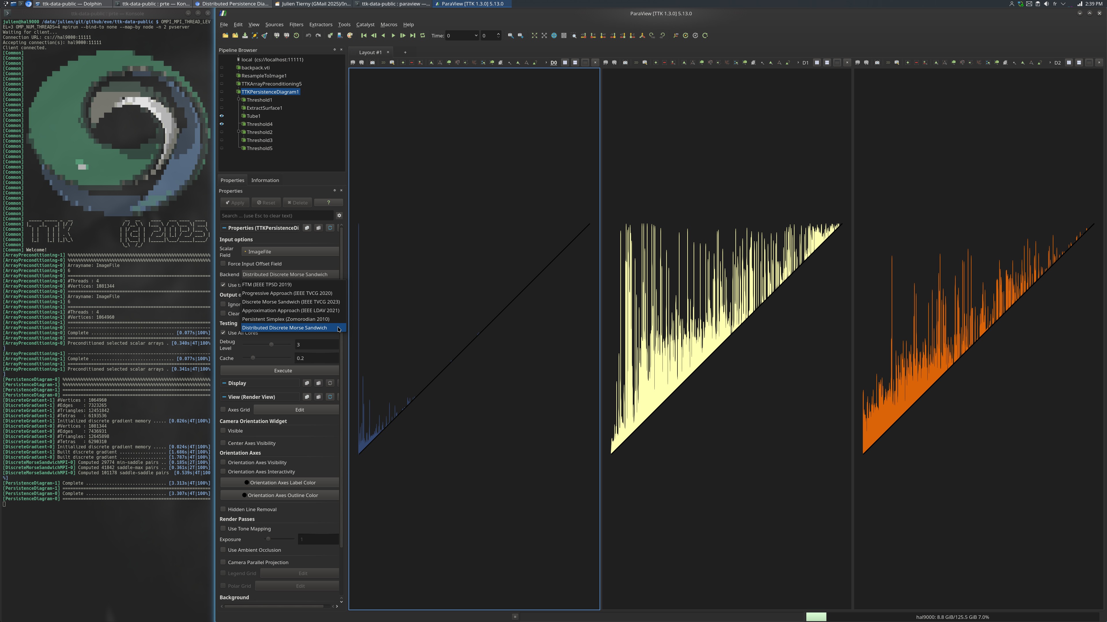
The produced visualization captures the persistence diagrams of each dimension ($D_0$, $D_1$ and $D_2$, from left to right in the image).

First, the data is loaded and the grid is resampled (to $128^3$ by default).

Then, a global ordering of the vertices is computed using the filter ArrayPreconditioning. This step will be triggered automatically if not explicitly called.

Then, the persistence diagram is computed via PersistenceDiagram and more specifically the Distributed Discrete Morse Sandwich algorithm (specified in the choice of software backend). Note that, in the output, each MPI process will create a dummy pair modeling the diagonal, which may need to be filtered out prior to subsequent processing (e.g., Wasserstein distance computation). This is achieved by the last step of the pipeline, involving thresholding (see the Python code below).

ParaView

To reproduce the above screenshot on 2 processes and 4 threads, go to your ttk-data directory and enter the following command:

OMPI_MPI_THREAD_LEVEL=3 OMP_NUM_THREADS=4 mpirun --bind-to none --map-by node -n 2 pvserver 

In another command line enter the following command:

paraview 

Now, follow the procedure described in paragraph $8.2.2$ of the following ParaView documentation to connect your ParaView server to your client. Once that is done, you can open the state file states/distributedPersistenceDiagram.pvsm in the ParaView GUI through File > Load State.

Python code

#!/usr/bin/env python

from paraview.simple import *

if len(sys.argv) == 2:
    dim = int(sys.argv[1])
else:
    dim = 128

# create a new 'XML Image Data Reader'
backpack = XMLImageDataReader(FileName=["backpack.vti"])

# create a new 'Resample To Image'
resampleToImage1 = ResampleToImage(Input=backpack)
resampleToImage1.SamplingDimensions = [dim, dim, dim]
resampleToImage1.SamplingBounds = [0.0, 511.0, 0.0, 511.0, 0.0, 372.0]

tTKArrayPreconditioning = TTKArrayPreconditioning(Input=resampleToImage1)
tTKArrayPreconditioning.PointDataArrays = ["ImageFile"]

# create a new 'TTK PersistenceDiagram'
tTKPersistenceDiagram1 = TTKPersistenceDiagram(Input=tTKArrayPreconditioning)
tTKPersistenceDiagram1.ScalarField = ["POINTS", "ImageFile"]
tTKPersistenceDiagram1.Backend = "Distributed Discrete Morse Sandwich"

# remove the dummy pairs representing the diagonal
threshold1 = Threshold(Input=tTKPersistenceDiagram1)
threshold1.Scalars = ['CELLS', 'PairType']
threshold1.UpperThreshold = 0.0
threshold1.ThresholdMethod = 'Above Upper Threshold'

UpdatePipeline()

# To save the output to disk, uncomment the line below.
# SaveData('diagram.pvtu', proxy=threshold1)

# WARNING: due to a reported ParaView issue, when saving the output to disk in
# MPI mode, pvbatch will execute the pipeline twice in a row (instead of one).

To run the above Python script using 4 threads and 2 processes, go to your ttk-data directory and enter the following command:

OMPI_MPI_THREAD_LEVEL=3 OMP_NUM_THREADS=4 mpirun --bind-to none --map-by node -n 2 pvbatch python/distributedPersistenceDiagram.py 

By default, the dataset is resampled to $128^3$. To resample to a higher dimension, for example $256^3$, enter the following command:

OMPI_MPI_THREAD_LEVEL=3 OMP_NUM_THREADS=4 mpirun --bind-to none --map-by node -n 2 pvbatch python/distributedPersistenceDiagram.py 256

Be aware that this may require too much memory to execute on a regular laptop.

Performance timing

Disclaimer

The distributed computation of persistence diagram has been evaluated on Sorbonne Universite's supercomputers. Therefore, the parameters of our algorithm have been tuned for this system and they might yield slightly different performances on a different supercomputer.

Run configuration

When using the above Python script with pvbatch, please make sure to adjust to your hardware the number of processes (-n option) and threads (OMP_NUM_THREADS variable). Note that TTK will default to a minimum number of 2 threads (to account for one communication thread) if the variable OMP_NUM_THREADS is set to a value smaller than 2.

For optimal performances, we recommend to use as many MPI processes as compute nodes (mapping one MPI process per node, see the --map-by node option in the above command line), and as many threads as (virtual) cores per node (in conjunction with the --bind-to none option in the above command line). Also, for load balancing purposes, we recommend to use a number of processes (-n option) which is a power of 2 (e.g., 2, 4, 8, 16, 32, 64, etc.).

Measuring time performance

For a precise time performance measurement, TTK needs to be built with the advanced CMake option TTK_ENABLE_MPI_TIME enabled.

In the terminal output, the full execution time of the distributed persistence computation (excluding IO) can be obtained by summing the times reported by the three following steps (4.11599 seconds overall in this example):

• [ArrayPreconditioning-0] Array preconditioning performed using 2 MPI processes lasted: 0.047390
• [DiscreteGradient-0] Computation performed using 2 MPI processes lasted: 2.172824
• [DiscreteMorseSandwichMPI-0] Computation of persistence pairs performed using 2 MPI processes lasted: 1.895776

Using another dataset

To load another dataset, replace the string backpack.vti in the above Python script with the path to your input VTI file and run the script with pvbatch as described above.

Inputs

• backpack.vti: A CT scan of a backpack filled with items.

Output

• diagram.pvtu: the persistence diagram of the backpack dataset.

C++/Python API

ArrayPreconditioning

PersistenceDiagram