Topology ToolKit

Writing a TTK module:
An introduction with Betti numbers

The purpose of this exercise tutorial is threefold:
   ·  Introduce you to the usage of TTK in ParaView;
   ·  Introduce you to the development of a TTK module;
   ·  Make you learn more about the homology groups of 3-manifolds in R3!

This exercise requires some minor background in C++.
It should take no more than 2 hours of your time.

1. Downloads

In the following, we will assume that TTK has been installed successfully on your system. If not, please visit our installation page for detailed instructions HERE.
Before starting the exercise, please download the data package HERE as well as the latest TTK source tree THERE.
Move the tarballs to a working directory (for instance called ~/ttk) and decompress them by entering the following commands (omit the $ character) in a terminal (this assumes that you downloaded the tarballs to the ~/Downloads directory):

$ mkdir ~/ttk
$ mv ~/Downloads/ttk-0.9.2.tar.gz ~/ttk/
$ mv ~/Downloads/bettiData.tar.gz ~/ttk/
$ cd ~/ttk
$ tar xvzf ttk-0.9.2.tar.gz
$ tar xvzf bettiData.tar.gz

You can delete the tarballs after the source trees have been decompressed by entering the following commands:

$ rm ttk-0.9.2.tar.gz
$ rm bettiData.tar.gz

2. TTK/ParaView 101

ParaView is the leading application for the interactive analysis and visualization of scientific data. It is open-source (BSD license). It is developed by Kitware, a prominent company in open-source software (CMake, CDash, VTK, ITK, etc.).

ParaView is a graphical user interface to the Visualization ToolKit, a C++ library for data visualization and analysis, also developed in open-source by Kitware.
VTK and ParaView both implement a pipeline model, where the data to analyze and visualize is passed on the input of a (possibly complex) sequence of elementary processing units, called filters. Each filter is implemented by a single C++ class in VTK. In ParaView, users can design advanced processing pipelines by placing manually each filter in their pipelines.
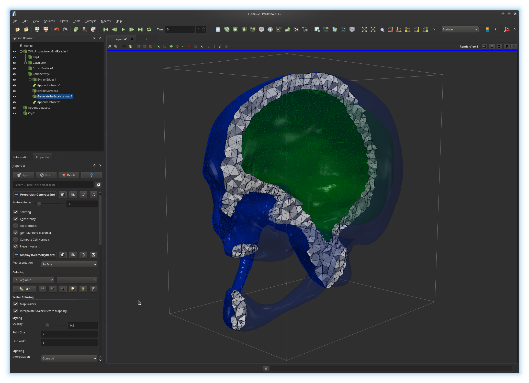
In the above example, the active pipeline (shown in the "Pipeline Browser", upper left panel) can be interpreted as a series of processing instructions and reads similarly to some source code: first, the input PL 3-manifold is clipped (Clip1); second, the boundary of the input PL 3-manifold is extracted (ExtractSurface1), third the connected components of the boundary are isolated and clipped with the same parameters as the rest of the volume (Clip2).

The output of each filter can be visualized independently (by toggling the eye icon, left column). The algorithmic parameters of each filter can be tuned in the "Properties" panel (bottom left panel) by selecting a filter in the pipeline (in the above example GenerateSurfaceNormals1). The display properties of the output of a filter in the main central view can also be modified from this panel.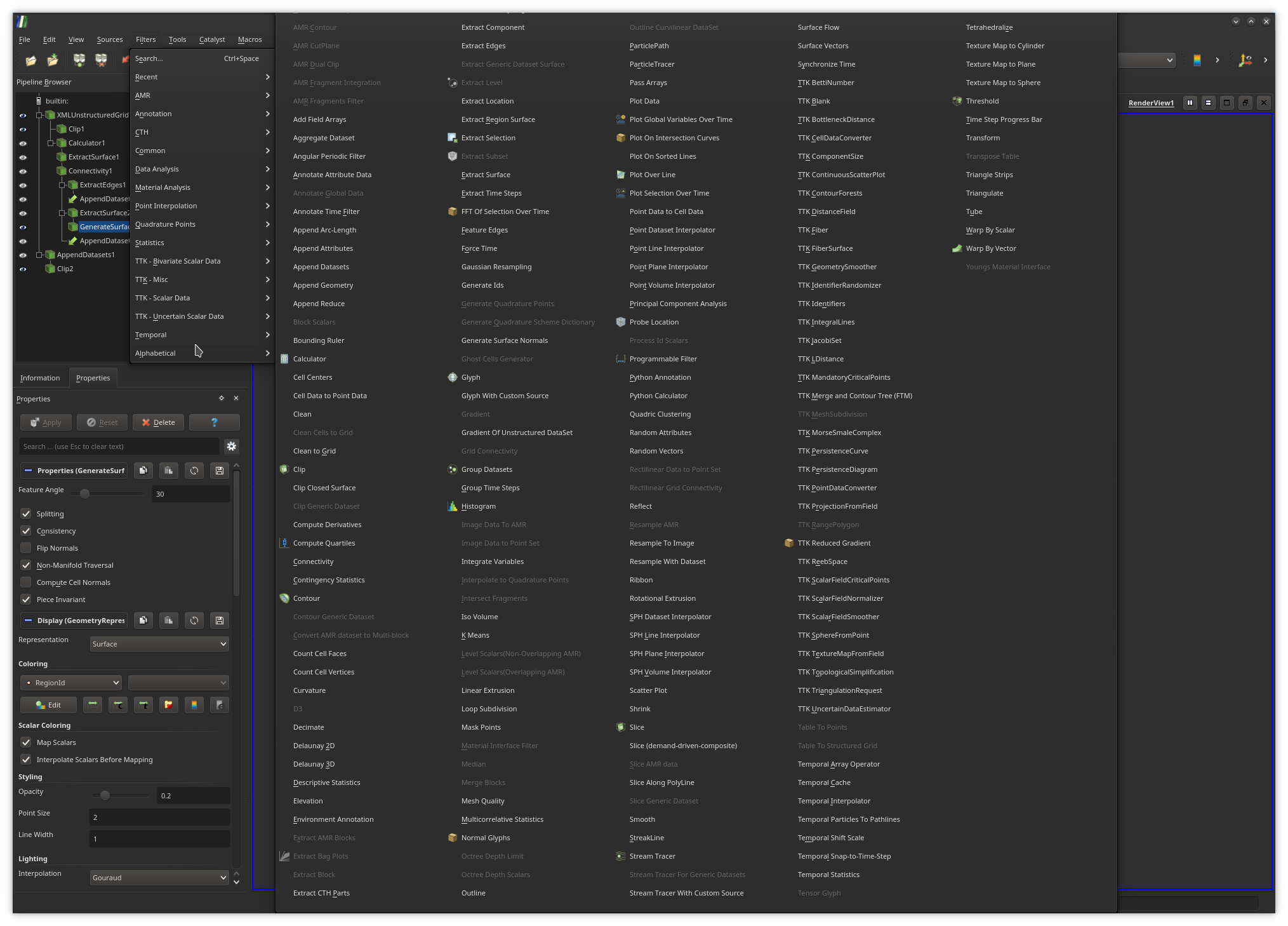
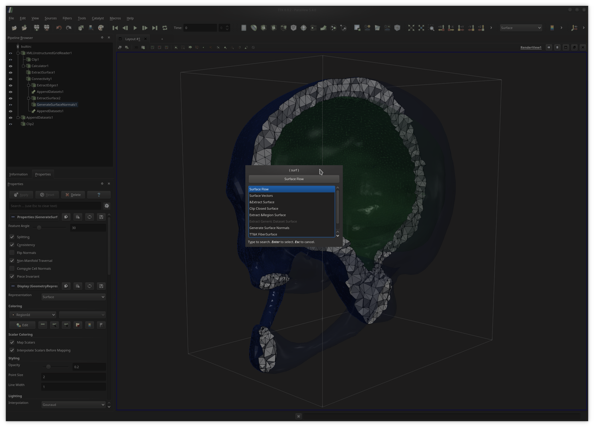
To create a pipeline from scratch, users typically load their input data and apply successively the required filters, by browsing the filter menu (exhaustive list shown above), where the filters which are not compatible with the object currently selected in the pipeline are shaded.
Alternatively to the filter menu, users can toggle a fast search dialog by pressing the Ctrl+space keystroke (under Linux) and enter keywords as shown above to quickly call filters.

Once users are satisfied with their analysis and visualization pipeline, they can save it to disk for later re-use in the form of a Python script with the menu File, Save state... and choosing the Python state file type. In the Python script, each filter instance is modeled by an independent Python object, for which attributes can be changed and functions can be called.
Note that the output Python script can be run independently of ParaView (for instance in batch mode) and its content can be included in any Python code (the pvpython interpreter is then recommended). Thus, ParaView can be viewed as an interactive designer of advanced analysis Python programs. Then, writing up your own TTK module will not only expose your C++ code to ParaView, but it will also make it readily available in Python. To learn more about the available ParaView filters, please see the following tutorials: HERE and THERE.

Exercise 1

Open the skull data set in ParaView with the following command (omit the $ character):

$ paraview ~/ttk/bettiData/skull.vtu

Next, try to reproduce the visualization shown in the first screenshot above, which shows a clipped view of the PL 3-manifold, with the visible interior triangles in white with dark edges, each boundary component displayed with its edges with a distinct color and the rest of the (unclipped) boundary shown in transparent.

3. Betti numbers of PL 3-manifolds

In the following, you will write your first TTK module, dedicated to the computation of Betti numbers of PL 3-manifolds. For this, we will exploit the results by Dey and Guha, published in their 1998 paper "Computing Homology Groups of Simplicial Complexes in R3".

Go ahead and create your TTK module by entering the following commands (omit the $ character):

$ cd ~/ttk/ttk-0.9.2/
$ scripts/createTTKmodule.sh BettiNumbers

The above script will create all the files and classes of your TTK module. This module includes automatically generated standalone command line and GUI programs, as well as a ParaView plugin.

For this exercise, we will only need to build your TTK module, and not the entire TTK collection. Thus, edit the file ~/ttk/ttk-0.9.2/CMakeLists.txt to remove all entries, except the first line and all the lines containing the word BettiNumbers.
Now, to build your TTK module, enter the following commands, where N is the number of available cores on your system (omit the $ character):

$ cd ~/ttk/ttk-0.9.2/
$ mkdir build
$ cd build
$ cmake ../
$ make -jN

Note that, in order to rebuild your module in the future, you'll only need to enter the last command (make -jN).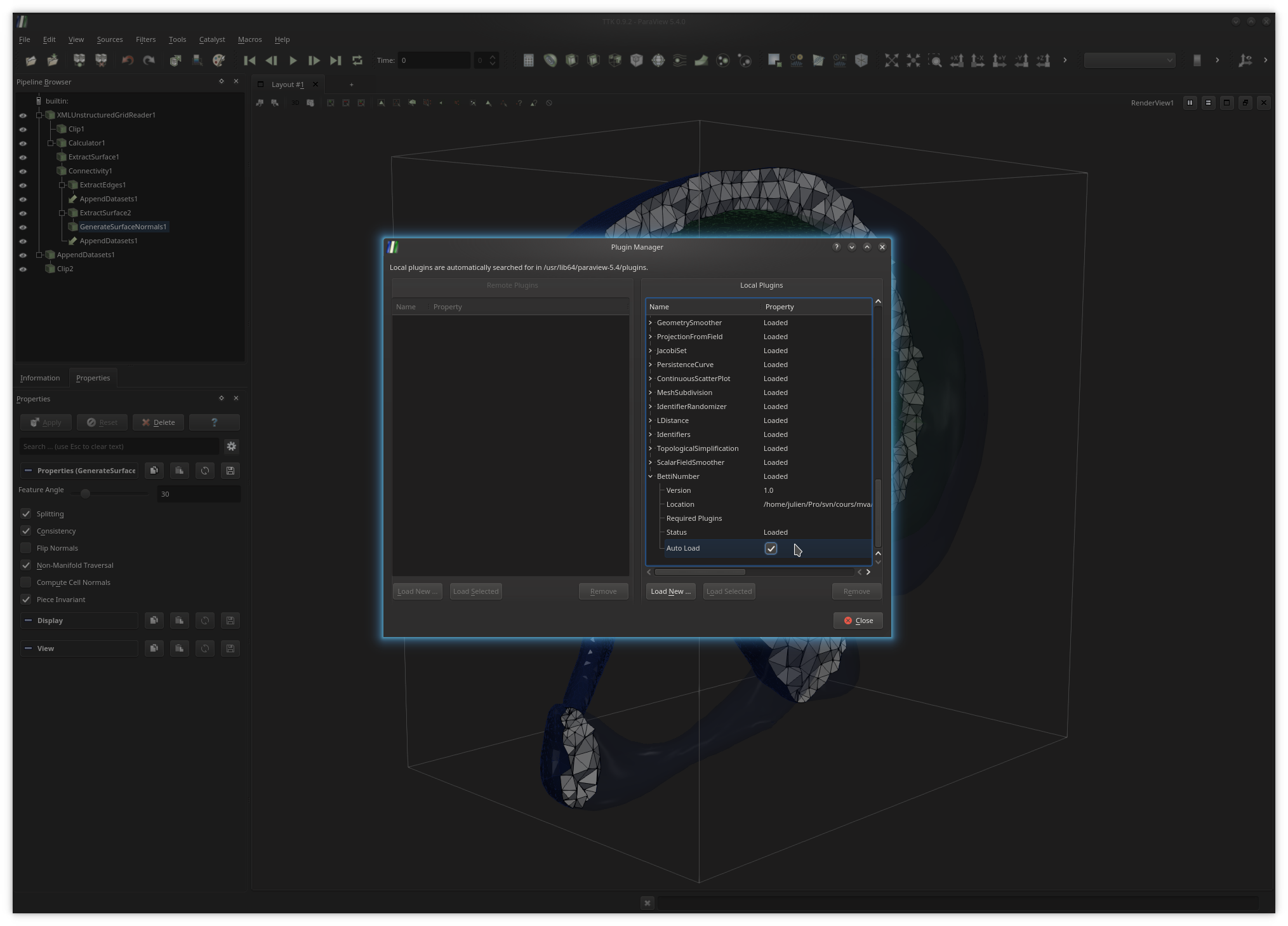
To load your module in ParaView, open ParaView, go to the menu Tools, Manage Plugins..., then click on the Load New... button. Next, from the file browser dialog, select the library we've just built: ~/ttk/ttk-0.9.2/build/paraview/BettiNumbers/libBettiNumbers.so. Next, you may want to check the checkbox AutoLoad as shown above (available after expending your plugin entry) to force ParaView to automatically load your plugin at startup.
At this point, if your plugin was successfully loaded, it should appear as the entry TTK BettiNumbers under the menu Filters then TTK - Misc, as shown below.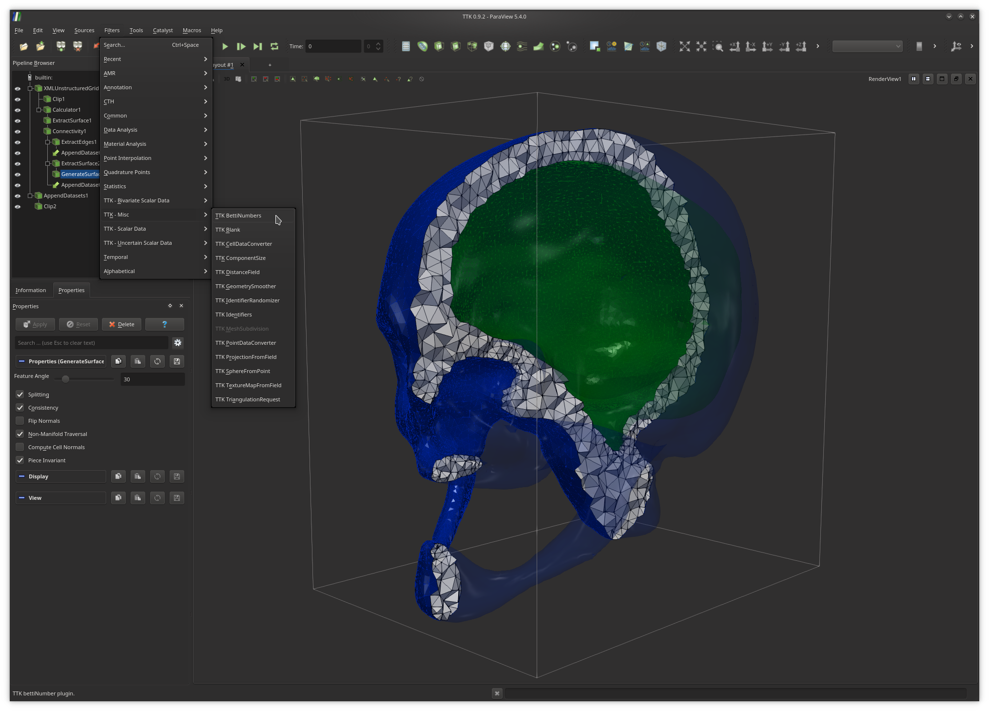
Now open the file ~/ttk/ttk-0.9.2/core/baseCode/bettiNumbers/BettiNumbers.h. In the function execute(), add the line cout << endl << "Hello World!" << endl << endl; before the return statement. Now build your module again, load the skull data set in ParaView and apply your BettiNumbers plugin. You should see your message "Hello World!" appear in the terminal, as shown below.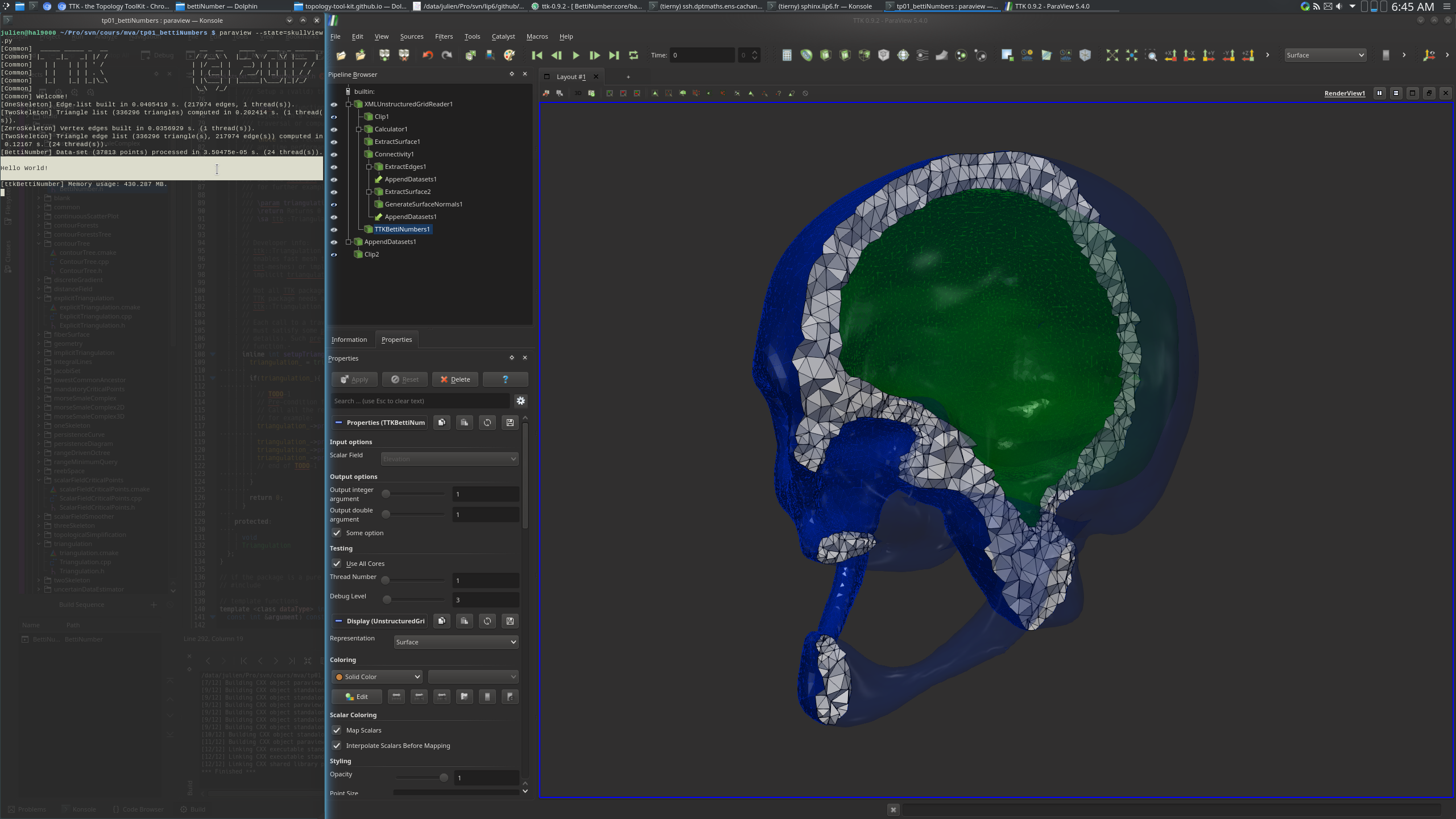
If this is the case, congratulations! You've just written your first TTK module!

Exercise 2: B0 (~20 lines of code)

The 0-th Betti number (noted B0) corresponds to the number of connected component of the input manifold M. In the following, we will compute this number and display it in the output of the terminal (next to our "Hello World!" message).

Several algorithms exist to enumerate connected components in a triangulation, the simplest being a simple breadth-first search traversal. Instead, we will use a Union-Find data-structure, which will make the implementation even simpler.

The Union-Find (UF) data-structure is a simple, yet powerful data-structure which tracks the connectivity of a graph over successive edge additions. It is a fundamental object which plays a key role in many computational topology algorithms.

Initially, a UF object is created for each vertex of the graph. The operation find() on this object returns its parent, that is a unique representative UF object which represents the connected component of the queried vertex.

When adding an edge between two vertices v0 and v1, the makeUnion() operation is called between the UF objects of v0 and v1. This will have the effect of merging the representatives of the corresponding connected components.

Thus, to enumerate the connected components of a PL manifold M, one just needs to proceed as follows. First, one should iterate over the edges of M, call the makeUnion() operation between the UF objects of the vertices of each edge of M. Finally, one should iterate over all the UF objects, call the find() operation and enumerate the number of unique remaining representatives. This number corresponds to the number of remaining connected components after all edges have been added (initially, the number of connected components is equal to the number of vertices in M).

TTK provides a reference implementation of the Union-Find data structure (with path compression and union by rank), which we will use in this exercise. Its online documentation can be found HERE.

To use it in your module, edit the file ~/ttk/ttk-0.9.2/core/baseCode/bettiNumbers/bettiNumbers.cmake and add the line ttk_add_baseCode_package(unionFind) at the top of the file. Next, in ~/ttk/ttk-0.9.2/core/baseCode/bettiNumbers/BettiNumbers.h, add the line #include <UnionFind.h> in the file preamble.

TTK provides an efficient data structure for fast triangulation traversal. Its online documentation can be found HERE.

In ~/ttk/ttk-0.9.2/core/baseCode/bettiNumbers/BettiNumbers.h, a pointer to an object of this class (triangulation_) is readily available and correctly initialized to the triangulation passed on the input of your module.

TTK's triangulation data-structure supports a cache based access. This means the data-structure needs to be pre-conditioned depending on the type of traversal it will undergo, before it gets actually traversed. For instance, if you want to access the i-th vertex of the j-th edge of the triangulation (with the function getEdgeVertex()), you will need, before the actual traversal, to call the pre-conditioning function preprocessEdges() in a pre-process, as explained in the documentation of the getEdgeVertex() function. Note that each traversal function comes with its own pre-conditioning function, to be called in the pre-processing stage of your module.

Typically, in ~/ttk/ttk-0.9.2/core/baseCode/bettiNumbers/BettiNumbers.h, the function setupTriangulation() is the right placeholder to put such a pre-conditioning statement, while the actual traversal should happen in the execute() function, next to our prior "Hello World!" message.

Now go ahead and compute B0, the number of connected components of M.

To do this, you'll need to allocate an array (typically an STL vector) of UnionFind objects with as many entries as vertices in M. Next, you'll need to iterate over the edges of M and call the makeUnion() operation on the UF objects of each edge. Finally, you'll need to iterate over your initial array of UF objects, re-assign to each entry the result of its find() operation (to obtain the latest representative) and enumerate the number of unique remaining representatives.

Exercise 3: B2 (~30 lines of code)

The 2-nd Betti number (noted B2) corresponds to the number of voids of the input manifold M. To compute B2, we will exploit one of the results by Dey and Guha, published in their 1998 paper "Computing Homology Groups of Simplicial Complexes in R3".

Parse the above paper and identify the expression of B2. From there, edit the function execute() of ~/ttk/ttk-0.9.2/core/baseCode/bettiNumbers/BettiNumbers.h to also compute and display B2.

Exercise 4: B1 (~20 lines of code)

The 1-st Betti number (noted B1) corresponds to the number of independent cycles of the input manifold M. To compute B1, we will exploit one of the results by Dey and Guha, published in their 1998 paper "Computing Homology Groups of Simplicial Complexes in R3".

Parse the above paper and identify the expression of B1. From there, edit the function execute() of ~/ttk/ttk-0.9.2/core/baseCode/bettiNumbers/BettiNumbers.h to also compute and display B1.

Exercise 5: Euler characteristic and beyond (~3 lines of code)

Compute and display the Euler characteristic X of M. How does it relate to the Betti numbers of M?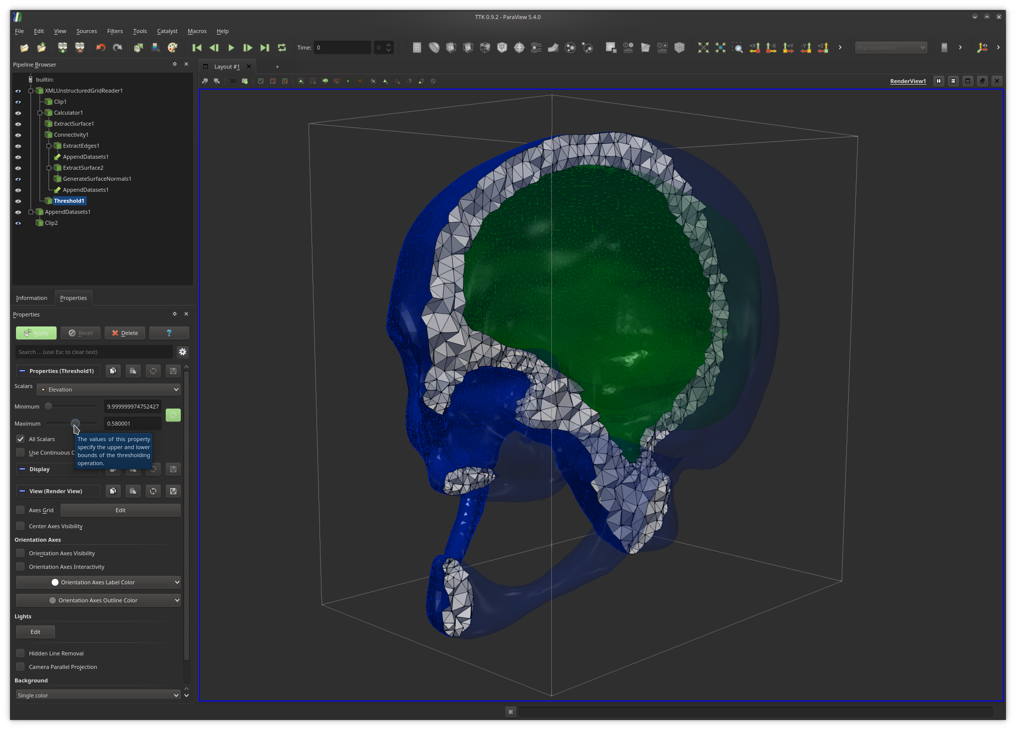
Now, in ParaView, use the Threshold filter on your input triangulation and modify the Maximum parameter (the upper bound). Since our test data sets come with an attached scalar field, this will have the effect of selecting all the tetrahedra of M with vertices having a default scalar value below the Maximum parameter.

Now use your module to compute the Betti numbers of this selection. Now adjust the Maximum parameter again and click on Apply. The Betti numbers should be updated automatically.

Keep on modifying the value Maximum. Where do the Betti numbers change? What do these configurations correspond to?

Check your intuition with the other data-sets available in the ~/ttk/bettiData/ directory. Note that for at.vti, you will need to call the filter Tetrahedralize prior to any other processing.

Now, instead of changing the Maximum parameter of the Threshold filter, change the Minimum parameter instead. What do you observe in terms of the changes of Betti numbers?