Interaction sites

Pipeline description

This example demostrates how topological analysis can be used to identify interaction sites i.e. different kind of chemical bonds in molecules. Using simulations and experiments, the electron density field denoted as Rho can be estimated for a molecule. Topological analysis of this scalar field can reveal important features in the data. For example, the maxima of this field correspond to the atom locations while saddles occur along the covalent bonds. However, for identification of non-covalent interactions like ionic bonds, analysis of the density field Rho is not enough. A derived scalar field from Rho called reduced density gradeint denoted by s is suggested in literature which can reveal non-covalent interation sites in a molecule. In this example, we will extract and compare the critical points for the Rho and s scalar fields for a simple molecule 1,2-ethanediol.

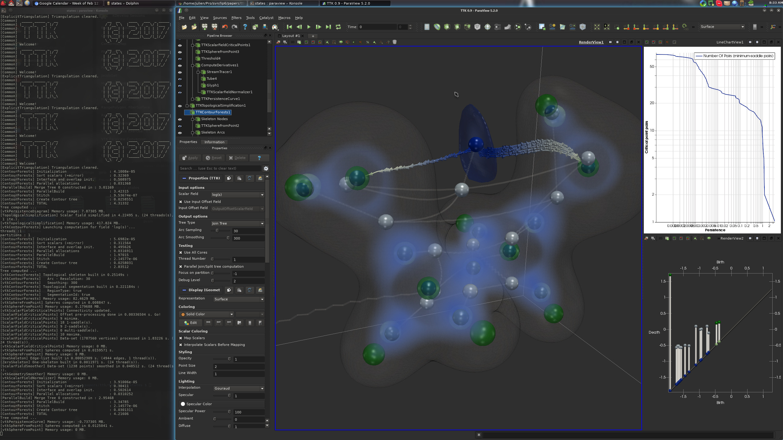
First a VTI file is loaded which contains two scalar fields namely log(Rho) and log(s). Then using ScalarFieldCriticalPoints, the critical points for log(Rho) are computed which are then converted into spheres using IcospheresFromPoints. They are shown as bigger transluscent green and white spheres in the screenshot above. Note that these critical points identify the atoms and covalent bonds in the molecule.

Next, we analyse log(s), the reduced gradient scalar field. Here, the PersistenceCurve is computed (top right view in the above screenshot). Then, the PersistenceDiagram for log(s) is computed and thresholds are applied based on persistence to maintain only the most persistent features. This results in a simplified persistence diagram (bottom right view in the above screenshot).

The simplified persistence diagram is then used as a constraint for the TopologicalSimplification of the input scalar data. The simplified data is then used as input to MergeTree to compute the join tree for the data. The join tree captures the topological changes in sub-level sets of the scalar field and therefore consists of leaves corresponding to minima and internal nodes corresponding to saddles, the points where sublevel sets merge. The nodes of this join tree are selected and highlighted as smaller opaque blue and white spheres using IcospheresFromPoints. Similarly, the arcs of the join tree are also extracted and shown as thin grey tubes in the screenshot above.

Using topological analysis of log(s), we identify an outlying minimum which is not close to the atom locations. This corresponds to a non-covalent interaction site in the molecule which is not identifiable using direct toplogical analysis of electron density field Rho. Lastly, we extract the segmented region corresponding to this particular minimum (shown as transluscent blue surface in the screenshot).

ParaView

To reproduce the above screenshot, go to your ttk-data directory and enter the following command:

paraview states/interactionSites.pvsm

Python code

#### import the simple module from the paraview
from paraview.simple import *

# create a new 'XML Image Data Reader'
builtInExamplevti = XMLImageDataReader(FileName=["BuiltInExample2.vti"])

#### Topological analysis of 'log(Rho)'

# extract the critical points using 'TTK ScalarFieldCriticalPoints'
tTKScalarFieldCriticalPoints1 = TTKScalarFieldCriticalPoints(Input=builtInExamplevti)
tTKScalarFieldCriticalPoints1.ScalarField = ["POINTS", "log(Rho)"]

# covert these points to spheres using 'TTK IcospheresFromPoints'
tTKIcospheresFromPoints3 = TTKIcospheresFromPoints(Input=tTKScalarFieldCriticalPoints1)
tTKIcospheresFromPoints3.Radius = 3.0

#### Topological analysis of 'log(s)'

# compute the 'TTK PersistenceDiagram'
tTKPersistenceDiagram1 = TTKPersistenceDiagram(Input=builtInExamplevti)
tTKPersistenceDiagram1.ScalarField = ["POINTS", "log(s)"]

# compute the 'TTK PersistenceCurve'
tTKPersistenceCurve1 = TTKPersistenceCurve(Input=tTKPersistenceDiagram1)

# create a new 'Threshold'
threshold1 = Threshold(Input=tTKPersistenceDiagram1)
threshold1.Scalars = ["CELLS", "PairIdentifier"]
threshold1.ThresholdMethod = "Between"
threshold1.LowerThreshold = 0.0
threshold1.UpperThreshold = 999999999

# remove low persistence critical points using 'Threshold'
persistenceThreshold = Threshold(Input=threshold1)
persistenceThreshold.Scalars = ["CELLS", "Persistence"]
persistenceThreshold.ThresholdMethod = "Between"
persistenceThreshold.LowerThreshold = 0.5
persistenceThreshold.UpperThreshold = 999999999

# simplify the field using 'TTK TopologicalSimplification'
tTKTopologicalSimplification1 = TTKTopologicalSimplification(
    Domain=builtInExamplevti, Constraints=persistenceThreshold
)
tTKTopologicalSimplification1.ScalarField = ["POINTS", "log(s)"]

# create a new 'TTK Merge and Contour Tree' to compute the join tree
tTKJoinTree1 = TTKMergeTree(Input=tTKTopologicalSimplification1)
tTKJoinTree1.ScalarField = ["POINTS", "log(s)"]
tTKJoinTree1.TreeType = "Join Tree"
tTKJoinTree1.ArcSampling = 30

# covert the critical points to spheres using 'TTK IcospheresFromPoints'
tTKIcospheresFromPoints4 = TTKIcospheresFromPoints(Input=tTKJoinTree1)
tTKIcospheresFromPoints4.Radius = 2.0

# extract the join tree arcs and save them as tubes
tTKGeometrySmoother2 = TTKGeometrySmoother(Input=OutputPort(tTKJoinTree1, 1))
tTKGeometrySmoother2.IterationNumber = 300

# create a new 'Extract Surface'
extractSurface4 = ExtractSurface(Input=tTKGeometrySmoother2)

# create a new 'Tube'
tube5 = Tube(Input=extractSurface4)
tube5.Radius = 0.25

# Extract the segmentation region corresponding to the interaction site
threshold6 = Threshold(Input=OutputPort(tTKJoinTree1, 2))
threshold6.Scalars = ["POINTS", "RegionType"]

# create a new 'Threshold'
threshold7 = Threshold(Input=threshold6)
threshold7.Scalars = ["POINTS", "SegmentationId"]
threshold7.ThresholdMethod = "Between"
threshold7.LowerThreshold = 13.0
threshold7.UpperThreshold = 13.0

# create a new 'Extract Surface'
extractSurface5 = ExtractSurface(Input=threshold7)

# create a new 'Tetrahedralize'
tetrahedralize1 = Tetrahedralize(Input=extractSurface5)

# create a new 'TTK GeometrySmoother'
tTKGeometrySmoother3 = TTKGeometrySmoother(Input=tetrahedralize1)
tTKGeometrySmoother3.IterationNumber = 10

# save the output
SaveData("logRhoCriticalPoints.vtp", tTKIcospheresFromPoints3)
SaveData("logSPersistenceCurve.csv", OutputPort(tTKPersistenceCurve1, 0))
SaveData("logSPersistenceDiagram.vtu", tTKPersistenceDiagram1)
SaveData("logSJoinTreeCriticalPoints.vtp", tTKIcospheresFromPoints4)
SaveData("logSJoinTreeArcs.vtp", tube5)
SaveData("NonCovalentInteractionSite.vtu", tTKGeometrySmoother3)

To run the above Python script, go to your ttk-data directory and enter the following command:

pvpython python/interactionSites.py

Inputs

• BuiltInExample2.vti: 3D scalar fields corresponding to electron density distribution Rho and the reduced density gradient s around a simple molecule 1,2-ethanediol.

Outputs

• logRhoCriticalPoints.vtp: All the scalar field critical points computed for log(Rho).
• logSPersistenceCurve.csv: The output persistence curve for log(s).
• logSPersistenceDiagram.vtu: The output persistence diagram for log(s).
• logSJoinTreeCriticalPoints.vtp: The critical points in the join tree of log(s).
• logSJoinTreeArcs.vtp: The arcs of the join tree of log(s).
• NonCovalentInteractionSite.vtp: The non-covalent interaction site region identified using the join tree of log(s).

Note that you are free to change the VTK file extensions to that of any other supported file format (e.g. csv) in the above python script.

C++/Python API

MergeTree

GeometrySmoother

IcospheresFromPoints

PersistenceCurve

PersistenceDiagram

ScalarFieldCriticalPoints

TopologicalSimplification